Why do we need interpretability?
Machine learning models have been widely adopted in the decision-making process in many critical domains; some uses include (i) determining whether a person receives loan from the bank, or (ii) modeling who is more likely to commit a crime. From these uses, it is clear that machine learning models have a large impact on people’s lives; therefore, it is imperative that machine learning models be well understood and free of any biases and discrimination. This idea of understanding the machine learning models underlies our definition of model interpretability.
Some models like linear regression and decision tree are inherently easy to interpret because we can easily inspect the contribution of each feature and know how each decision was made. Other models like Neural Networks or Random Forest, however, are complex and much harder to interpret. This high complexity in a lot of machine learning models on one hand means they can be applied to many complicated tasks such as image classification, but on the other hand, it also means that there is a need for an interpretability method to understand these black box models in a faithful and human-friendly manner.
The most popular methods for interpreting black box models are the local, model-agnostic methods. In the next section, I will introduce two local model-agnostic perturbation-based interpreability methods: LIME and SHAP.
Model-Agnostic Perturbation-based Interpretability Methods
First, let’s talk a little bit about the vocabulary here. Model-agnostic methods mean that the methods will work for any “black box”, no matter whether the black box is a deep neural network or a random forest. A model-agnostic interpretability model, therefore, does not assume anything about the machine learning model that it is trying to explain.
Now, what does perturbation-based mean? Perturbation-based interpretability models aims to estimate feature contribution by looking at perturbations around a given instance and observe the effect of those perturbations on the output.
Here is the set-up for the perturbation-based interpretability method:
-
$f$: model we’re trying to explain
-
$g$ a simpler model that can be interpreted
-
$\pi_x(x’)$: similarity function between the given instance $x$ and the perturbed instance $x’$
-
$\Omega(g)$: complexity function of the model $g$
The interprability method aims to find the best linear model $g$ that is low in complexity and that best approximates $f$ around the given instance $x$. The algorithm can be formalized as follows [3, 4]:
\[\arg \min_{\text{linear model}\ g} L(f,g,\pi_x) + \Omega(g),\]where the loss function $L$ is defined as:
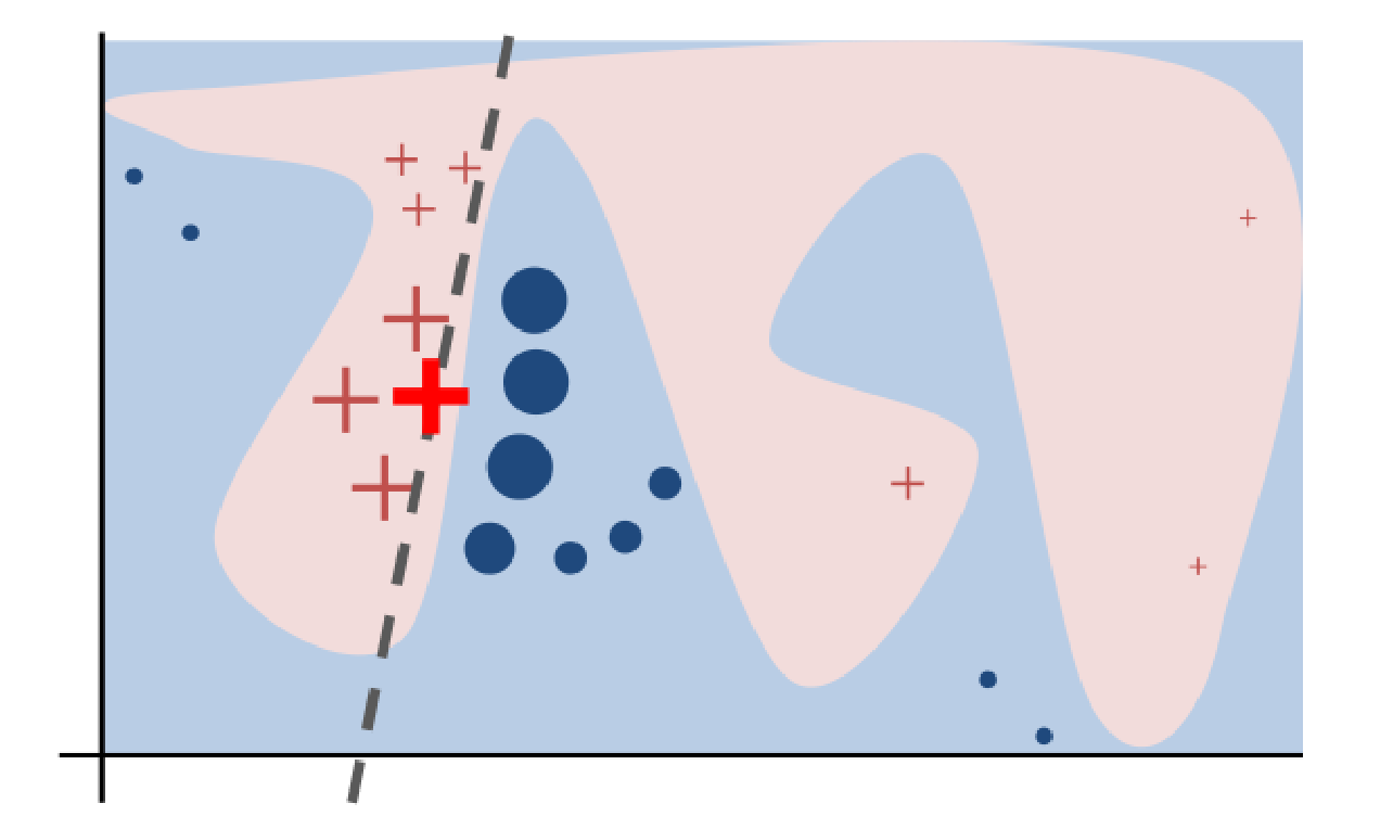
\[\begin{equation} L(f,g,\pi_x) = \sum_{x'} [ f(x') - g(x') ]^2 \pi_x(x'). \end{equation}\]Let us talk a little bit about the two equations above. In Equation (2), note that the distance between the classifier $f$ and the linear model $g$ is weighted by the similarity of the given instance $x$ and the perturbed instance $x’$. This term means that for points close to the given instance $x$, we want the model $g$ to approximate $f$ closely; conversely, for points that are far away from $x$, we don’t really care if $g$ is similar to $f$. This property is called local fidelity – model $g$ is trying to approximate $f$ locally around instance $x$.
Note that as $g$ gets more complex, it can better approximate $f$. However, in Equation (1), we notice the term $\Omega(g)$, which makes sure that $g$ is as interpretable as possible. The terms in Equation (1) best summarizes the fidelity-interpretability trade-off.
Two of the most popular interpretability methods are LIME and SHAP. The differences between LIME and SHAP lie in how $\Omega$ and $\pi_x$ are chosen:
-
LIME uses $L^2$ norm for similarity function $\pi_x$ and the number of non-zero weights for $\Omega$.
-
SHAP uses Shaply values from Game Theory for $\Omega$.
LIME
Here is a visual representation of how LIME works [3]:
SHAP
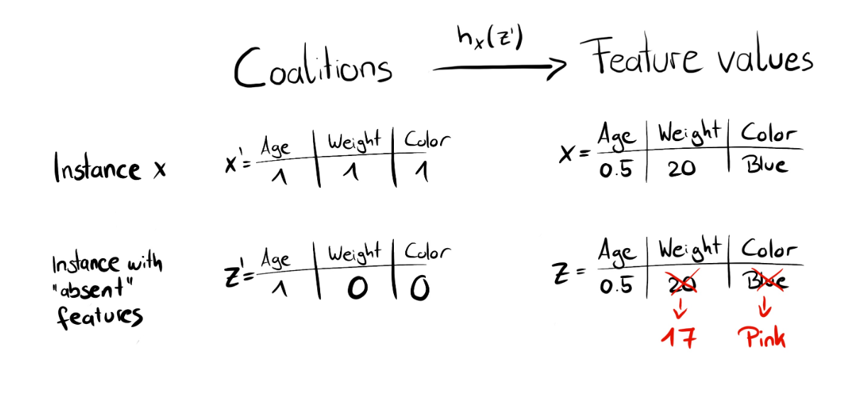
Instead of using $L^2$ distance, SHAP uses another metric from Game Theory. Here’s how SHAP works: to get the importance of feature $S[i]$:
-
Get all subsets of features $S$ that do not contain $S[i]$
-
Compute the effect of our predictions of adding $S[i]$ to all those subsets
$\Rightarrow$ Super computationally expensive.
Here are some examples of how SHAP works [2]:
Attacks on Perturbation-based Models
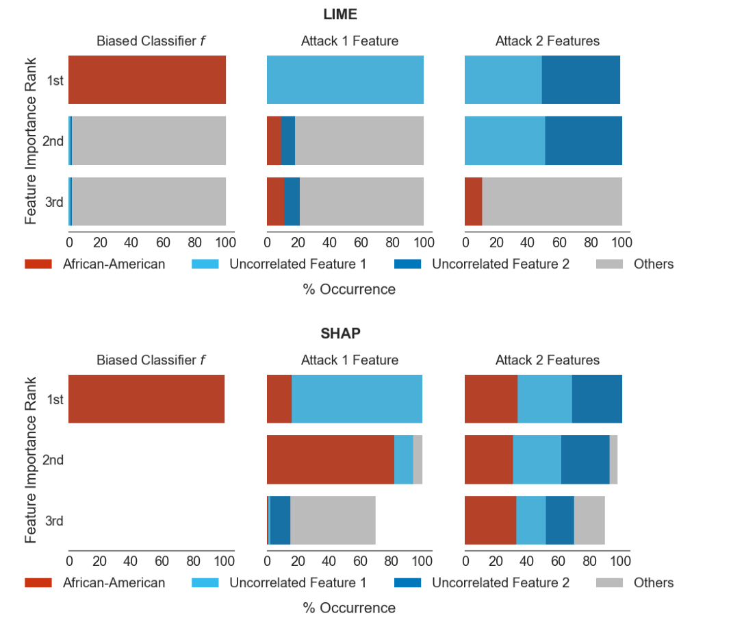
Drawback of LIME and SHAP: depends on random sampling of new points. Attackers can make the biased black box appear innocent on the perturbed data points.
Note that by perturbing points, a lot of points will not have the same distribution as the original dataset. Idea of the attacks: build a classifier that is biased on the dataset distribution $\mathcal{D}$ but innocent-looking on points that are not in the distribution (so that LIME and SHAP won’t detect the biases).
Results of the attack [4]:
References
[1] Scott M Lundberg and Su-In Lee. “A Unified Approach to Interpreting Model Predictions”. In: Advances in Neural Information Processing Systems 30. Ed. by I. Guyon et al. Curran Associates, Inc., 2017, pp. 4765–4774. url: http://papers.nips.cc/paper/7062-a-unified-approach-to-interpreting-model-predictions.pdf (visited on 02/10/2020).
[2] Christoph Molnar. 5.7 Local Surrogate (LIME). Interpretable Machine Learning. url: https://christophm.github.io/interpretable-ml-book/lime.html (visited on 02/16/2020).
[3] Marco Tulio Ribeiro, Sameer Singh, and Carlos Guestrin. “”Why Should I Trust You?”: Explaining the Predictions of Any Classifier”. In: arXiv:1602.04938 [cs, stat] (Aug. 9, 2016). arXiv: 1602.04938. url: http://arxiv.org/abs/1602.04938 (visited on 02/08/2020).
[4] Dylan Slack et al. “Fooling LIME and SHAP: Adversarial Attacks on Post hoc Explanation Methods”. In: arXiv:1911.02508 [cs, stat] (Feb. 3, 2020). arXiv: 1911.02508. url: http://arxiv.org/abs/1911.02508 (visited on 02/08/2020).